A Spectral Renormalization-Group View of Learning
This research draft develops a Wilsonian renormalization-group (RG) view of neural-network layer convergence. It connects three ideas that have usually been discussed separately: Heavy-Tailed Self-Regularization (HTSR), the SETOL statistical-mechanics theory, and optimizer-induced spectral flow.
The central proposal is that strong trained layers approach a scale-balanced spectral boundary near α ≈ 2. Statistically, this is where learning reaches the edge of non-self-averaging. In RG power counting, it is the marginal point where equal logarithmic spectral bands contribute comparable energy. The same construction explains the SETOL trace-log condition through the retained-coordinate Jacobian and motivates RG-aware optimizer corrections such as WW-PGD.
- α > 2: stable, but the learned heavy tail can be too weak.
- α ≈ 2: scale-balanced, maximally structured before dominant-tail takeover.
- α < 2: tail modes or correlation traps can dominate and increase overfitting risk.
- Tr log X̃R = 0: removes arbitrary retained-volume scale while preserving spectral shape.
Research draft: Charles H. Martin, PhD, Calculation Consulting, June 2026. | Read the draft PDF | GitHub staging copy | WeightWatcher GitHub
1 · The Theory in One Pass
Deep learning is normally described as loss minimization. This paper argues that a second object
is equally important: the internal spectral organization of each layer. For a dense layer
with weights W, define the layer correlation operator
The eigenvectors of X identify learned input directions; its eigenvalues measure the
gain assigned to those directions. During training, many layers move from a random-matrix-like
spectrum toward a heavy-tailed spectrum. The proposed RG description organizes that movement.
HTSR supplies the observation
Strong trained layers often develop heavy-tailed empirical spectral densities, and many good checkpoints sit near α ≈ 2.
SETOL supplies the effective space
SETOL connects layer quality to the empirical spectrum and selects a retained Effective Correlation Space (ECS) with a trace-log scale condition.
RG supplies the flow picture
Decimate tiny-eigenvalue noise, retain correlated modes, remove arbitrary scale, and test whether the normalized spectral shape approaches a stable endpoint.
1.1 · HTSR and SETOL identify the same layerwise endpoint
The paper argues that two diagnostics that were originally developed for different purposes actually point to the same converged layer state. HTSR fits the heavy-tailed part of the empirical spectral density and finds that well-trained layers often sit near \(\alpha\approx 2\). SETOL independently selects an effective correlation space and tests whether its normalized retained spectrum lies on the trace-log gauge slice, \(\sum_{i=1}^{\widetilde M}\log \widetilde\lambda_i \approx 0\). The proposed fixed-point picture is that both conditions hold simultaneously for a good layer.
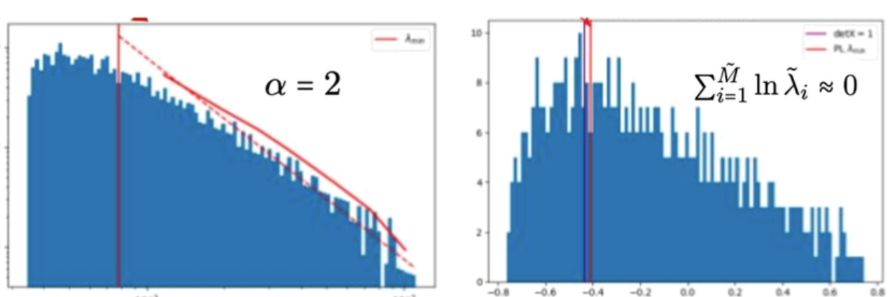 Representative endpoint diagnostics from the paper. Left: the HTSR power-law fit gives
\(\alpha \approx 2\). Right: the trace-log-normalized ECS satisfies
\(\sum_{i=1}^{\widetilde M}\log \widetilde\lambda_i \approx 0\). The theory proposes that
strong layers satisfy both conditions at convergence.
Representative endpoint diagnostics from the paper. Left: the HTSR power-law fit gives
\(\alpha \approx 2\). Right: the trace-log-normalized ECS satisfies
\(\sum_{i=1}^{\widetilde M}\log \widetilde\lambda_i \approx 0\). The theory proposes that
strong layers satisfy both conditions at convergence.
2 · What Actually Flows?
The microscopic optimizer updates every entry of W, but the RG description does not
attempt to reproduce every weight-space detail. Instead it follows the retained empirical
spectral density. In shorthand,
One operational RG step has four parts: remove tiny-eigenvalue noise, retain the correlated ECS, rescale the retained operator, and test the remaining spectral energy and shape. The fixed-point object is not a raw matrix. It is an equivalence class of normalized retained spectra.
2.1 · Reading the spectral RG-flow schematic
The RG-flow schematic below summarizes how the paper interprets optimizer training as spectral evolution. The dashed blue line marks the ECS or trace-log boundary; the dashed red line marks the start of the MLE-fitted power-law tail. During useful training, these two independently selected cutoffs move toward one another. Near convergence they align, and the fitted slope approaches \(\alpha\approx 2\).
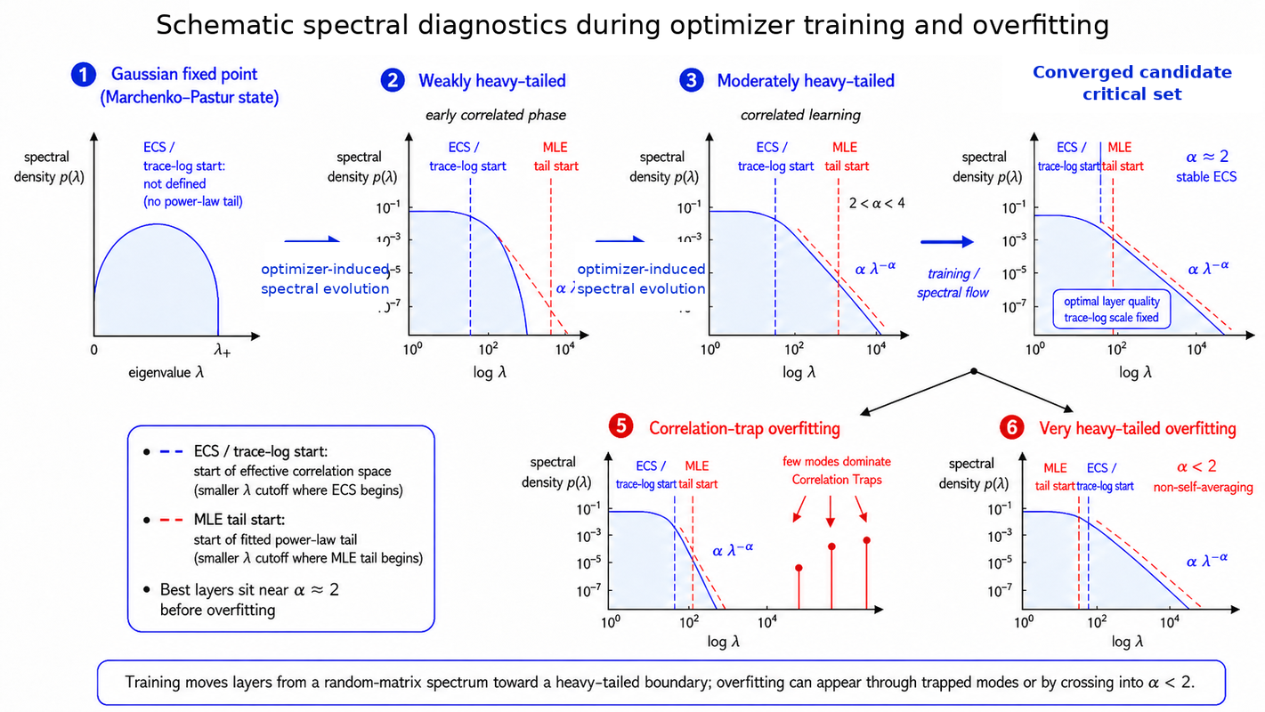 Schematic spectral diagnostics during optimizer training and overfitting. The flow starts from a
Gaussian random-matrix-like layer, passes through increasingly heavy-tailed structured states, and
can either converge near the proposed critical set or overshoot into two different overfitting modes.
Schematic spectral diagnostics during optimizer training and overfitting. The flow starts from a
Gaussian random-matrix-like layer, passes through increasingly heavy-tailed structured states, and
can either converge near the proposed critical set or overshoot into two different overfitting modes.
Panels 1–4: the intended training route
- Gaussian fixed point: no stable ECS or heavy-tailed tail is present yet.
- Weakly heavy-tailed: structure begins to form and the ECS cutoff appears before a mature power-law tail.
- Moderately heavy-tailed: correlated learning develops, and the spectrum carries a clearer heavy-tailed sector.
- Converged candidate critical set: the ECS boundary and fitted tail start align, while the layer sits near \(\alpha\approx 2\).
Panels 5–6: two ways to overfit
- Correlation-trap overfitting: a few trapped modes peel away and dominate even though the bulk tail may still look reasonable.
- Very heavy-tailed overfitting: the whole retained tail crosses into \(\alpha<2\), so dominant modes carry too much spectral weight and the layer becomes non-self-averaging.
In short, the image expresses the paper's main RG claim: training drives layer spectra away from the Gaussian fixed point toward a marginal heavy-tailed boundary. Good training stops near the aligned HTSR/SETOL critical set; overtraining pushes the spectrum into trap-dominated or very-heavy-tailed regimes.
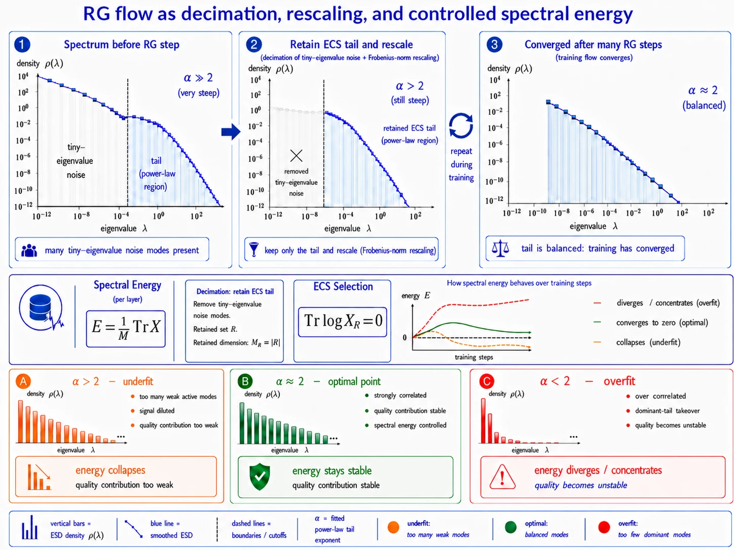 Operational spectral RG flow. Training removes weak modes, concentrates useful correlations in an
ECS, and can approach a balanced heavy-tailed shape near α ≈ 2.
Operational spectral RG flow. Training removes weak modes, concentrates useful correlations in an
ECS, and can approach a balanced heavy-tailed shape near α ≈ 2.
This is a layerwise fixed-point picture. A multilayer network need not have one global matrix fixed point. Each matrix-like layer has its own retained spectrum and must reach a compatible endpoint with the other layers.
3 · Why α = 2 Is Special
3.1 · Statistical meaning: the self-averaging boundary
A macroscopic observable is self-averaging when relative sample-to-sample fluctuations vanish
as the system grows. For an observable OM, the paper uses the relative variance
When \(\mathcal{V}_M(O) \to 0\), one sufficiently large sample becomes representative of the ensemble. When it stays finite, different data samples, random seeds, or training runs can remain measurably different. In a layer spectrum, this can happen through two mechanisms:
- Localized correlation traps: a few anomalous outlier modes dominate.
- Collective heavy-tailed fluctuations: many retained modes fluctuate coherently.
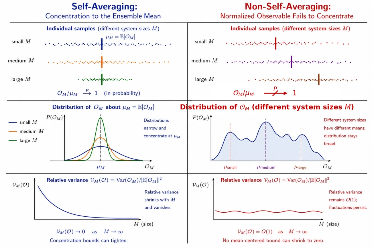 Self-averaging allows concentration bounds to tighten with scale. Non-self-averaging leaves a finite
normalized width, so a mean-centered bound need not become informative.
Self-averaging allows concentration bounds to tighten with scale. Non-self-averaging leaves a finite
normalized width, so a mean-centered bound need not become informative.
3.2 · RG meaning: equal energy per logarithmic scale
The leading retained spectral observable is the first moment of the normalized ECS spectrum, interpreted as a spectral energy:
Set \(x = \log \widetilde\lambda\). Since \(d\widetilde\lambda = \widetilde\lambda\,d\log\widetilde\lambda\), the energy carried by one logarithmic spectral scale is
α > 2
Energy per logarithmic band decreases toward the largest eigenvalues. The layer can be stable, but the learned tail may be too weak or underdeveloped.
α = 2
Every fixed-ratio spectral band carries comparable energy. This is the proposed marginal, scale-balanced boundary.
α < 2
Energy grows toward the dominant tail. A few large modes can carry an order-one fraction of the total and make the layer unstable or non-self-averaging.
4 · RG Power Counting in Detail
The derivative argument can be written as a finite-shell calculation. Take one multiplicative spectral shell \([\Lambda,b\Lambda]\), with fixed \(b>1\), and define the band energy
For a power-law tail \(\widehat\rho_R(\widetilde\lambda)=C\widetilde\lambda^{-\alpha}\),
The second expression is independent of \(\Lambda\). Moving the same fixed-ratio shell up or down the tail does not change its energy contribution. That is the cleanest form of the marginality claim.
4.1 · Running coupling, beta function, and scaling dimension
The paper uses the shell gain itself as a running spectral coupling,
For an exact power law, the leading spectral beta function and scaling dimension are
| Regime | Scaling dimension | Band-energy flow | Learning interpretation |
|---|---|---|---|
| α > 2 | yE < 0 |
Gain decreases with spectral scale. | Stable or self-averaging, but potentially undertrained or weakly correlated. |
| α = 2 | yE = 0 |
Gain is constant across logarithmic bands. | Marginal boundary; maximal stable structured variation before tail domination. |
| α < 2 | yE > 0 |
Gain grows toward the largest modes. | Dominant-tail sector; correlation traps and overfitting risk. |
5 · The Retained-Coordinate Jacobian and the Trace-Log Law
The trace-log condition is not inserted only as a normalization trick. It arises from the volume change
of the retained coordinate map. After an SVD/ECS decimation, let WR contain the
retained right-singular directions and map retained coordinates a to layer outputs:
Because WR can be rectangular, its ordinary determinant is not the relevant
object. The induced retained-volume factor comes from the Gram determinant:
Therefore the positive retained Jacobian is
Scale-invariant ERG gauge
Apply the same calculation to the normalized retained operator \(\widetilde X_R\). Requiring a unit retained volume gives
The trace-log is the additive log-volume coordinate removed by the gauge choice.
5.1 · What is fixed, and what is still allowed to flow?
Fixed by the gauge
- The retained product scale.
- The covariance-volume coordinate.
- The arbitrary multiplicative size of the retained operator.
Still free to flow
- The tail slope and fitted α.
- The first moment and band-energy distribution.
- The ECS support and dominant-tail burden.
- The normalized spectral shape.
This distinction is essential: the trace-log fixes scale; it is not itself the flowing spectral energy. The energy and tail shape remain physical observables after the redundant scale coordinate is removed.
6 · Redundant Directions and Quotient Spectral Flow
Wilsonian RG acts on equivalence classes rather than every microscopic coordinate. In the retained spectral description, two important motions can be redundant.
Trace-log or volume drift
The update changes the retained product scale and leaves the chosen gauge slice, even when the normalized spectral shape is nearly unchanged.
Isospectral coordinate motion
An orthogonal similarity transformation rotates retained coordinates while preserving the full eigenvalue multiset and the trace-log.
The trace-log correction removes one normal direction, but a similarity orbit lies tangent to the trace-log surface. Consequently, Tr log X̃R = 0 is necessary but not sufficient for a complete RG quotient.
There is also a network-level caveat. A rotation that is isospectral for one layer is not automatically redundant for the full neural network: it changes the coordinates sent to the next layer. It can be removed only when adjacent layers transform compatibly or a functional test verifies that the network output is unchanged.
7 · The Operational Fixed-Point Test
The paper uses “fixed point” operationally. It does not claim that one finite checkpoint is an exact closed-form solution of the complete network dynamics. A candidate fixed point is a normalized retained spectral shape that remains stable after final decimation and trace-log testing.
One practical RG step
- Compute the layer spectrum.
- Remove tiny-eigenvalue noise.
- Select a retained ECS.
- Apply Frobenius rescaling.
- Measure or restore the trace-log gauge.
- Compare the retained shape and energy with the previous step.
Candidate endpoint signature
- The SETOL ECS aligns with the independently fitted HTSR tail.
- The retained normalized ESD is stable.
- Tr log X̃R ≈ 0.
- α ≈ 2.
- A truncated-SVD layer restricted to the ECS preserves generalization.
8 · What the Theory Says About Optimizers
The supervised optimizer remains primary. RG-aware corrections should act on a completed optimizer proposal, remain local and damped, and fall back to the original update whenever the correction damages the loss trajectory or destabilizes the retained support.
8.1 · Muon as a crude approximation
Muon approximately orthogonalizes matrix-valued updates, replacing a strongly anisotropic update spectrum by one with nearly equal active singular values. In the RG interpretation, this can suppress excessive anisotropic scale motion. However, Muon does not select an ECS, compute the layer-state trace-log normal, or determine which isospectral directions are truly redundant for the full network.
8.2 · WW-PGD as a finite spectral retraction
WW-PGD is a first-pass experiment that tests the proposal more directly. A base optimizer proposes a finite layer matrix. WW-PGD then selects a working spectral window between the fitted power-law start and the trace-log ECS start, reshapes the rank-ordered tail toward an α ≈ 2 target, restores the selected trace-log, and blends the result back into the optimizer trajectory.
What WW-PGD controls
- One retained log-volume coordinate.
- The rank-order shape of a selected tail window.
- A soft homotopy toward the α ≈ 2 target.
- A post-correction residual used to weaken or skip unsafe corrections.
It does not implement the complete sampled isospectral quotient. It is an approximate, falsifiable test of the RG optimizer hypothesis.
9 · Preliminary Experimental Evidence
The present experiments are deliberately small. They use a three-layer MNIST MLP and track fitted WeightWatcher exponents across training. The results should be read as proof-of-concept evidence, not as a universal optimizer benchmark.
9.1 · AdamW versus Muon
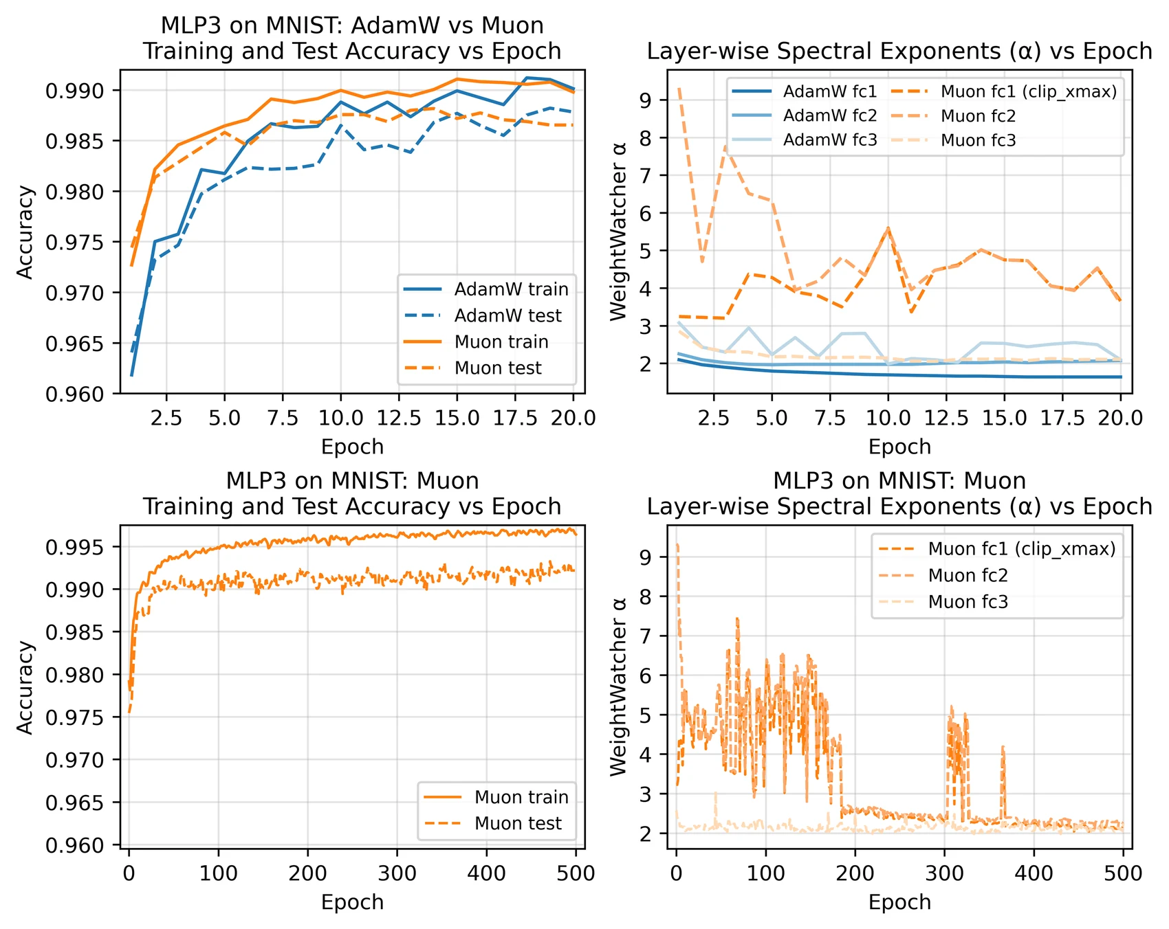 In the reported run, AdamW drives one layer below α = 2 early, while Muon follows a slower spectral route
and eventually moves the tested layer exponents toward the proposed boundary.
In the reported run, AdamW drives one layer below α = 2 early, while Muon follows a slower spectral route
and eventually moves the tested layer exponents toward the proposed boundary.
9.2 · WW-PGD on ordinary training
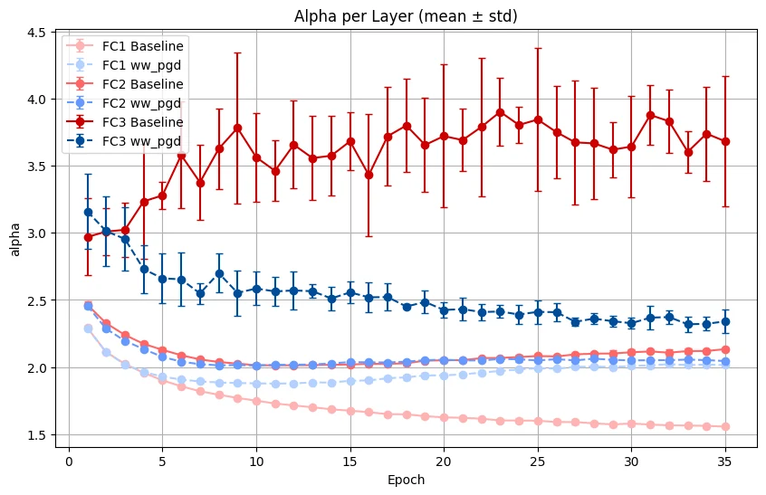 WW-PGD changes the layerwise spectral trajectories and pulls the tested layers toward the α ≈ 2
region.
WW-PGD changes the layerwise spectral trajectories and pulls the tested layers toward the α ≈ 2
region.
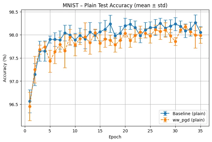 The spectral correction preserves approximately comparable test accuracy in the reported five-run
experiment.
The spectral correction preserves approximately comparable test accuracy in the reported five-run
experiment.
9.3 · Repairing an anti-grokking checkpoint
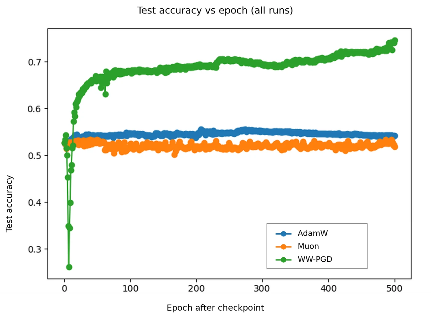 Starting from the selected overfit checkpoint, the preliminary WW-PGD run recovers substantially more
held-out accuracy than resumed AdamW or Muon.
Starting from the selected overfit checkpoint, the preliminary WW-PGD run recovers substantially more
held-out accuracy than resumed AdamW or Muon.
10 · Universality Beyond One Architecture
The broader conjecture is that different learning algorithms may follow different microscopic update rules while approaching similar coarse-grained spectral structure. The proposed universal observables would be measured near a candidate endpoint, not read directly from the raw parameterization.
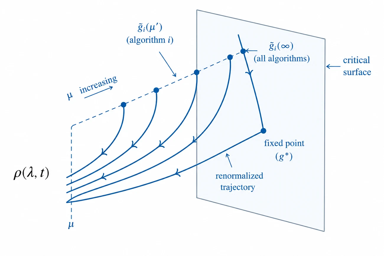 Candidate universality: different nonlinear learners can follow different microscopic trajectories yet
approach a common coarse-grained critical surface and spectral endpoint.
Candidate universality: different nonlinear learners can follow different microscopic trajectories yet
approach a common coarse-grained critical surface and spectral endpoint.
Neural networks provide the direct case because every matrix-like layer has an explicit correlation operator. For boosted trees and other nonlinear learners, one must first define an effective correlation operator—for example, a Gram matrix built from prediction increments—before the same spectral questions become testable.
Universality here does not mean that all algorithms compute the same function. It means that successful learners may share comparable coarse-grained spectral organization: stable bulk structure, controlled dominant modes, and a marginal balance between weak learning and overconcentration.
11 · What Is Established, and What Remains a Proposal?
Empirical or operational ingredients
- WeightWatcher measures layerwise ESDs and fitted heavy-tail exponents.
- Many strong models exhibit heavy-tailed layer spectra.
- Correlation traps can be tested by randomized-spectrum outliers.
- The ECS, trace-log residual, tail burden, and α can be tracked across checkpoints.
- The reported Muon and WW-PGD experiments can be reproduced and falsified.
Theoretical claims still under test
- That α ≈ 2 is a universal layerwise RG endpoint.
- That the self-averaging and marginality boundaries coincide broadly.
- That common optimizers converge to the proposed spectral fixed point.
- That a complete quotient optimizer can remove redundant directions safely.
- That the same universality class extends to boosted trees and other learners.
The paper’s value is therefore not only explanatory. It defines a concrete measurement program: track α, ECS-tail alignment, trace-log residuals, trap counts, and tail concentration across training; then ask whether generalization improves near the marginal boundary and degrades when the tail becomes dominant.
12 · Read the Draft and Related Work
The GitHub PDF is a temporary public copy while the manuscript is being prepared for archival release. Replace the staging link with the final arXiv or journal URL when available.